Flow Over Cylinder: Vortex Shedding Study

Background: Von Kármán Vortex Shedding

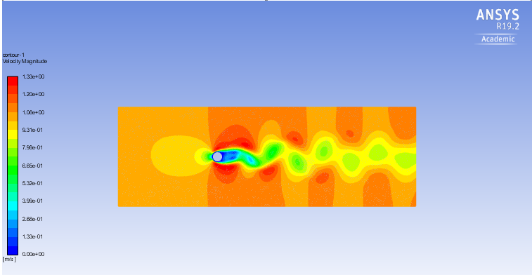
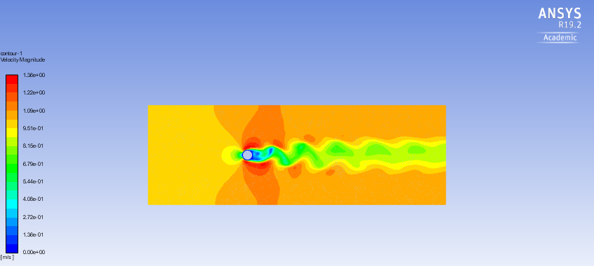
When a bluff body like a cylinder is placed in a uniform flow, the boundary layer separates periodically from the upper and lower surfaces, creating an alternating pattern of counter-rotating vortices downstream, a von Kármán vortex street.

This phenomenon governs:

Structural loading on offshore risers, bridge cables, and heat exchanger tubes, the periodic shedding creates oscillating lift forces that can drive resonance
Heat transfer, the vortex street enhances convective mixing downstream of the cylinder
Flow-induced noise, the shedding frequency sets the dominant acoustic tone in bluff-body flows

Von Kármán vortex streets form in laminar flow when 40 < Re < 100. Reynolds number is controlled here by fixing geometry and velocity while tuning dynamic viscosity.

Strouhal number (St) is the dimensionless measure of shedding frequency:

St = fL / U, where f = shedding frequency, L = characteristic length (cylinder diameter), U = free-stream velocity

St values between 0.2 and 0.4 indicate oscillation-dominated flow.

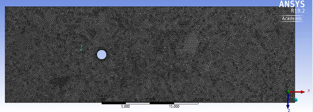
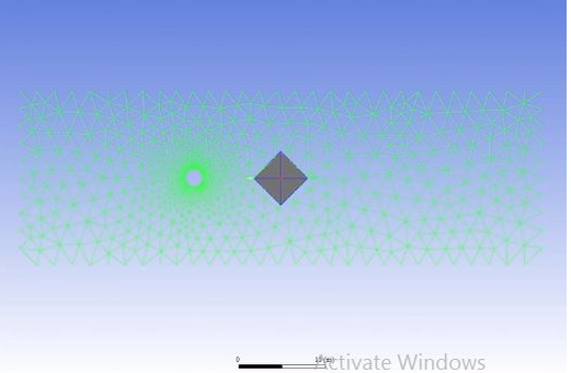
Mesh Setup

A triangular mesh was used throughout the domain to accurately resolve the curved cylinder surface and capture the vortex wake. An inflation layer was applied around the cylinder wall to increase near-wall resolution, critical for correctly predicting separation point and shedding onset.

Triangular mesh with inflation layer around cylinder — Triangular mesh with inflation layer around the cylinder. Finer cells near the wall capture the boundary layer; coarser cells away from the cylinder reduce computational cost.

Monitor point location, 10m downstream from cylinder centre — Monitor point placed 10 m downstream from the cylinder centre. Velocity history at this point is used to detect shedding onset and measure frequency.

Simulation Parameters

Parameter	Value
Cylinder diameter (L)	2 m
Free-stream velocity (U)	1 m/s
Air density (ρ)	1 kg/m³
Dynamic viscosity (μ)	0.02 kg/m·s
Reynolds number (Re)	100
Mesh element size	0.25 mm
Solver type	Pressure-based
Working fluid	Air

Re = ρUL/μ = (1 × 1 × 2) / 0.02 = 100, within the laminar vortex-shedding regime.

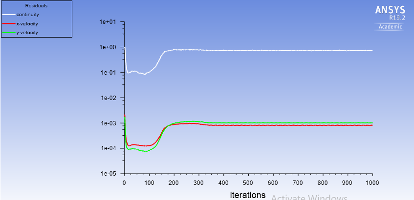
Case 1, Steady-State Solver

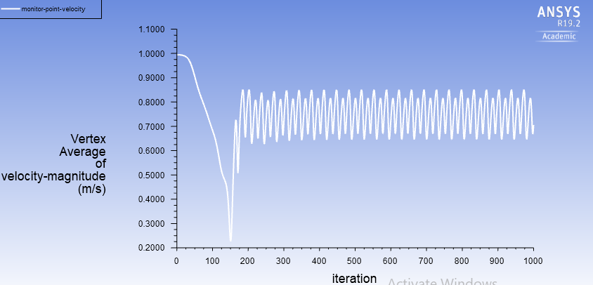
The steady-state solver computes a time-averaged solution. For vortex shedding problems this is a deliberate choice: a steady solver cannot properly converge an inherently unsteady flow, so the oscillations in the residuals and monitor signal reveal the shedding physics rather than hiding them.

Run: 1000 iterations

Case 1 steady-state residual plot, oscillating after 150 iterations — Residual plot, Case 1 (steady). Residuals decrease up to ~150 iterations then oscillate rather than converging, a signature of an unsteady flow being forced into a steady solver.

Case 1 velocity at monitor point, periodic oscillation indicating vortex shedding — Velocity magnitude at the downstream monitor point. The periodic rise-and-fall confirms vortex shedding even in steady mode, but the signal lacks a well-defined time axis, making Strouhal number calculation unreliable.

Case 1 velocity distribution, alternating vortex street downstream of cylinder — Velocity distribution across the domain at Re = 100. The alternating high- and low-velocity zones downstream of the cylinder clearly show the von Kármán vortex street. The asymmetry in the wake confirms that shedding is active.

Case 2, Transient Solver

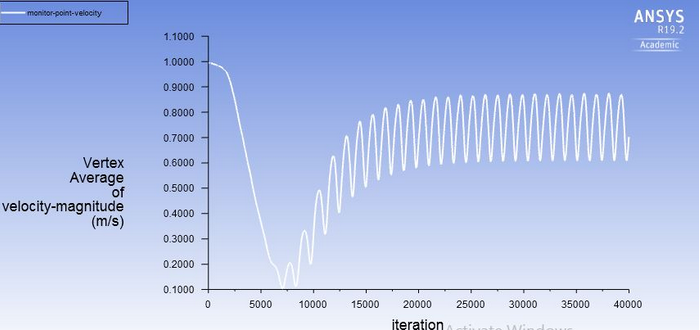
The transient solver resolves the time-dependent flow field step by step, capturing the actual vortex formation, growth, and shedding cycle. This is the physically correct approach for shedding problems and the only mode from which a meaningful Strouhal number can be extracted.

Case 2 transient residual plot — Residual plot, Case 2 (transient). The solver converges within each time step. The larger number of total iterations reflects the time-stepping approach, each iteration step advances the solution in time.

Case 2 velocity magnitude at monitor point vs iterations, vortex onset at ~8000 iterations — Velocity at monitor vs iteration count. Vortex shedding begins forming around 8,000 iterations; the pattern stabilises and becomes periodic after ~20,000 iterations.

Case 2 velocity magnitude vs flow time, periodic signal used to extract shedding frequency — Velocity vs flow time. Shedding begins at ~35 s and converges to a stable periodic signal after ~120 s. The steady oscillation period is used to extract the shedding frequency f = 11/60 Hz.

Case 2 transient vortex shedding, alternating vortices in the wake — Transient velocity field showing the fully developed von Kármán vortex street. Counter-rotating vortices alternate on each side of the wake, the hallmark pattern for Re = 100.

Results & Strouhal Number

Key findings

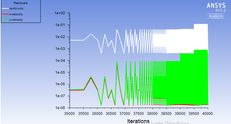
Steady solver detects shedding but cannot quantify it. The oscillating residuals and velocity monitor confirm that vortex shedding is occurring, but without a resolved time axis the shedding frequency cannot be reliably extracted, Strouhal number is indeterminate from steady results.

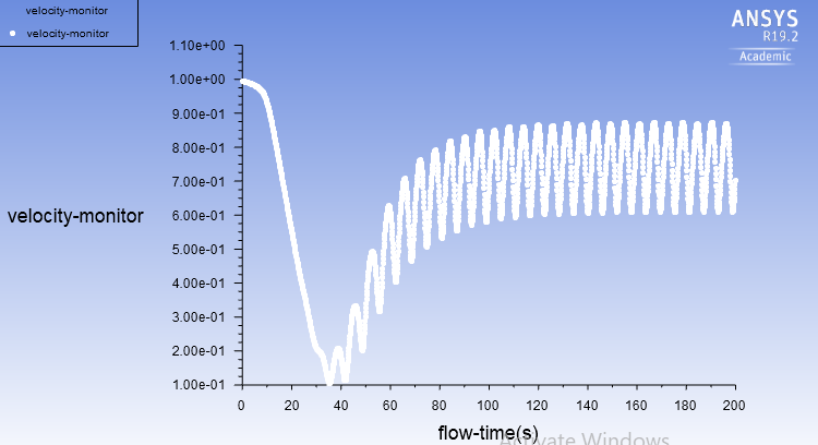
Transient solver resolves the shedding cycle fully. The velocity-time signal converges to a stable periodic oscillation after ~120 s of flow time, giving a clean frequency measurement.

Strouhal number confirms oscillation-dominated flow. St = 0.36 falls within the 0.2-0.4 range expected for Re = 100, validating both the mesh setup and the transient solver configuration.

Case	Solver	Shedding Visible	St Calculable	St Value
1	Steady-state	Yes (oscillating residuals)	No	,
2	Transient	Yes (resolved cycles)	Yes	0.36

Strouhal number calculation, Case 2:

f = 11/60 Hz · L = 2 m · U = 1 m/s

St = fL/U = (11/60 × 2) / 1 = 0.367 ≈ 0.36

Since 0.2 < St < 0.4 → oscillation dominates the flow, consistent with Re = 100 vortex-shedding regime.